Supporting code for phase-only compressive sensing (2/2)
Phase-Only Compressive Sensing
This notebook aims at testing the possibility to recovery a signal from phase-only observations, as described in the papers:
- [1] L. Jacques, T. Feuillen, “The importance of phase in complex compressive sensing”, 2020 (arXiv)
- [2] L. Jacques, T. Feuillen, “Keep the phase! Signal recovery in phase-only compressive sensing”, 2020 (arXiv)
The code relies on the “basis pursuit denoising” (BPDN) solver implemented by “SPGL1: A solver for sparse least squares”, and in particular its port to Python.
As described in [1,2], the phase-only compressive sensing is defined from the following model:
$$ \boldsymbol z = {\rm sign}_{\mathbb C}(\boldsymbol \Phi \boldsymbol x) \tag{PO-CS} $$
with ${\rm sign}_{\mathbb C}(\lambda) = \lambda/|\lambda|$ the complex sign operator, a complex Gaussian random matrix $\boldsymbol \Phi \sim \mathbb C \mathcal N^{m \times n}(0,2)$, and $\boldsymbol x$ an $k$-sparse vector in $\mathbb R^n$.
The papers above develop a method to recover, up to a global amplitude, $\boldsymbol x$ from $\boldsymbol z$.
Remark: All the codes below are based on a complex Gaussian matrix $\boldsymbol \Phi$. However, complex Bernoulli and random partial Fourier sensing are also implemented through the function generate_sensing_mtx(m,n,model='gaussian'), with model in {'gaussian','bernoulli','fourier'}. Feel free to play with them.
Requirements:
Preliminaries: Loading important modules. If you cannot run or install the progress bar of tqdm, just comment the lines where it’s used. See below.
import numpy as np
from scipy import interpolate
from scipy.sparse.linalg import LinearOperator

import matplotlib.pyplot as plt
import matplotlib.colors as mcolors
import matplotlib.cm as cm

#from scipy.sparse.linalg import LinearOperator
#from scipy.sparse import spdiags
import spgl1

# for nice progress bars (comment it if it doesn't work)
from tqdm.notebook import tqdm


# Initialize random number generators
np.random.seed(43273289)
%matplotlib inline
1. Noiseless PO-CS reconstruction
Let us define a few important functions, namely the complex sign operator ${\rm sign}_{\mathbb C}$, the constant $\kappa = \sqrt{\pi/2}$, the signal-to-noise ratio metric, as well as a shortcut to call the BPDN solver from SPGL1.
# numerical error constant: 10*np.finfo(np.float32).eps
epsilon = 10*np.finfo(np.float32).eps

# complex sign operator
signc = lambda x: x / (np.absolute(x) + (x == 0)*epsilon)

# the kappa constant (see [1])
kappa = np.sqrt(np.pi/2)

# the SNR metric between two signals (in dB)
snr = lambda a,b: 20*np.log10(np.linalg.norm(a)/np.linalg.norm(a-b))

# simplifying the call to BP from SPGL1 and storing parameters in the same time
#bpalg = lambda A, b: spgl1.spg_bp(A, b, opt_tol=1e-7, bp_tol=1e-7)[0]
#bpalg = lambda A, b: spgl1.spg_bp(A, b, opt_tol=1e-8, bp_tol=1e-8, iscomplex=False)[0]
bpalg = lambda A, b: spgl1.spg_bp(A, b, opt_tol=1e-7, bp_tol=1e-7)[0]

# simplifying the call to BPDN from SPGL1 and storing parameters in the same time
bpdnalg = lambda A, b, sigma: spgl1.spg_bpdn(A, b, sigma)[0]

# a function to generate the j^th canonical vector in d dimensions
def generate_canonic_vec(d,j):
    e_j = np.zeros(d)
    e_j[j] = 1.0
    return e_j
A function to generate real $k$-sparse signals in $\mathbb R^n$.
def generate_sparse_sig(k,n):
    idx = np.random.permutation(n)
    x = np.zeros(n)
    x[idx[0:k]] = np.random.randn(k)
    return x
Let’s define several functions generating $m \times n$ random sensing matrix constructions, namely complex Gaussian, complex Bernoulli, and partial Fourier random matrices.
def generate_complex_Gaussian_mtx(m,n):
    Phi = np.random.randn(m, n) + np.random.randn(m, n) *1j;
    A = Phi/np.sqrt(m)
    return A

def generate_complex_Bernoulli_mtx(m,n):
    Phi = np.sign(np.random.randn(m, n)) + np.sign(np.random.randn(m, n)) *1j;
    A = Phi/np.sqrt(m)
    return A

class generate_partial_Fourier_mtx(LinearOperator):
    def __init__(self, m, n):
        self.m = m
        self.n = n
        self.shape = (m, n)
        self.dtype = np.complex128
        self.idx = np.random.permutation(n)[0:m]

    def _matvec(self, x):
        z = np.fft.fft(x) / np.sqrt(self.m)
        return z[self.idx]

    def _rmatvec(self, y):
        z = np.zeros(self.n, dtype=complex)
        z[self.idx] = y
        return np.fft.ifft(z) * self.n / np.sqrt(self.m)

def generate_sensing_mtx(m,n,model='gaussian'):
    if model == 'gaussian':
        return generate_complex_Gaussian_mtx(m,n)
    elif model == 'bernoulli':
        return generate_complex_Bernoulli_mtx(m,n)
    elif model == 'fourier':
        return generate_partial_Fourier_mtx(m,n)
    else:
        print("unknown model")
A function to turn complex linear operators (applied to real vectors) into real linear operators with two times as many rows.
class Op2Real(LinearOperator):
    def __init__(self, A):
        self.A = A
        m, n = A.shape
        self.shape = [2*m, n]
        self.dtype = np.float64

    def _matvec(self, x):
        return np.concatenate(((self.A @ x).real,
                               (self.A @ x).imag))

    def _rmatvec(self, y):
        m = self.A.shape[0]
        return (self.A.T @ y[0:m]).real + (self.A.T @ y[m:]).imag
Following [1], this function constructs the equivalent matrix $\boldsymbol A_{\boldsymbol z}$ from both the phase measurements $\boldsymbol z$ and the sensing matrix $\boldsymbol A$.
class generate_Az(LinearOperator):
    def __init__(self, A, z):
        self.A = A
        self.ismat = (type(A) == np.ndarray)
        self.z = z
        self.D = np.diag(z)
        self.shape = (A.shape[0]+2, A.shape[1])
        self.dtype = np.float64

    def _matvec(self, x):

        m = self.A.shape[0]
        n = self.A.shape[1]

        H_z_x = self.D.conj().T @ (self.A @ x)

        alpha_adj_x = np.array([np.ones(m) @ H_z_x / (kappa * np.sqrt(m))])

        return np.concatenate([alpha_adj_x.real, alpha_adj_x.imag, H_z_x.imag])

    def _rmatvec(self, y):
        # passed the adjoint test
        m = self.A.shape[0]
        n = self.A.shape[1]

        if self.ismat:
            alpha = (self.A.conj().T @ (self.D @ np.ones(m))) / (kappa * np.sqrt(m))
            return (alpha.real * y[0]) - (alpha.imag * y[1]) - (self.A.conj().T @ (self.D @ y[2:])).imag

        else:
            alpha = (self.A.H @ (self.D @ np.ones(m))) / (kappa * np.sqrt(m))
            return (alpha.real * y[0]) - (alpha.imag * y[1]) - (self.A.H @ (self.D @ y[2:])).imag
1.1 Single reconstruction
We can now define the sensing model.
# Dimensions
n = 128 # space dimension
m = 50  # number of measurements
k = 10  # sparsity level

# Generating the complex Gaussian matrix
#A = generate_complex_Gaussian_mtx(m,n)
sensing_model = 'gaussian'

A = generate_sensing_mtx(m, n, model = sensing_model)

# Generating a k-sparse signal, random k-length support, and Gaussian entries
x = generate_sparse_sig(k,n)

# Linear measurements
y = A @ x

# Phase only measurements
z = signc(y)

# Definition of the matrix A_z for sparse signal recovery in PO-CS, such that A_z x0 = (1, 0, ..., 0)
A_z = generate_Az(A,z)

#A_z = build_Az(A,z)

# Let x0 such that ||Ax0||_1 = kappa sqrt(m) (see [1])
# This is the signal we hope to estimate, as the amplitude of x is lost (see [1])
x0 = x * kappa * np.sqrt(m) / np.linalg.norm(y,1)

# The measurement vector e_1 such that A_z x0 = e_1
e_1 = generate_canonic_vec(m+2,0)
We can compute that $|\boldsymbol A \boldsymbol x_0 - \boldsymbol e_1|$ is 0, up to numerical errors:
print(f"||Ax0||_1 = {np.linalg.norm(A @ x0,1)/(kappa*np.sqrt(m))}")
print(f"||Ax0 - e_1|| = {np.linalg.norm((A_z @ x0) - e_1)}")
||Ax0||_1 = 1.0000000000000002
||Ax0 - e_1|| = 2.056073113926681e-16
We now solve the linear and phase-only basis pursuit (BP) problems, defined by, respectively
$$ \boldsymbol x_{\rm lin} \in \arg\min_{\boldsymbol u} |\boldsymbol u|_1\ {\rm s.t.}\ \boldsymbol A \boldsymbol u = \boldsymbol y, \tag{BP/Lin} $$
$$ \boldsymbol x_{\rm PO-CS} \in \arg\min_{\boldsymbol u} |\boldsymbol u|_1\ {\rm s.t.}\ \boldsymbol A_z \boldsymbol u = \boldsymbol e_1, \tag{BP/PO-CS} $$
rembering that $\boldsymbol x_{\rm lin}$ should estimate $\boldsymbol x$, and $\boldsymbol x_{\rm PO-CS}$ should estimate $\boldsymbol x_0$.
# Linear model (note: running SPGL1 on complex mtx seems wrong).
A_equiv = Op2Real(A)
y_equiv = A_equiv @ x
x_lin = bpalg(A_equiv, y_equiv)

# Phase-only model
x_pocs = bpalg(A_z, e_1)

# SNRs
print(f"The SNR between x_lin and x is {snr(x_lin, x):.4} dB")
print(f"The SNR between x_pocs and x0 is {snr(x_pocs,x0):.10} dB")
The SNR between x_lin and x is 138.6 dB
The SNR between x_pocs and x0 is 110.8458148 dB
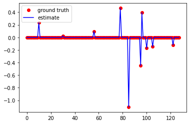
plt.figure()
plt.plot(x0, 'ro', label="ground truth")
plt.plot(np.real(x_pocs), 'b', label="estimate")
plt.legend()
<matplotlib.legend.Legend at 0x12d4540d0>
1.2 Systematic analysis over a range of measurements
Let’s now try a range of different measurements over many trials to see when the linear and the phase-only methods succeed
# sensing model
sensing_model = 'gaussian'

# Dimensions
n = 256
k = 20
m_vec = np.arange(1,256,10)
nb_trials = 100

# Inits
scores_lin = np.zeros((m_vec.size,nb_trials))
scores_po = np.zeros((m_vec.size,nb_trials))

# Main Monte Carlo Loop
pbar = tqdm(total=m_vec.size) #comment this if it doesn't work for you
for m_ind, m in enumerate(m_vec):

    # The measurement vector e_1 such that A_z x0 = e_1
    e_1 = generate_canonic_vec(m+2,0)

    for s in np.arange(nb_trials):

        # Generating the sensing matrix according to the selected model
        A = generate_sensing_mtx(m, n, model = sensing_model)

        # Generating a k-sparse signal, random k-length support, and Gaussian entries
        x = generate_sparse_sig(k,n)

        # Linear measurements
        y = A @ x

        # Phase only measurements
        z = signc(y)

        # Definition of the matrix A_z for sparse signal recovery in PO-CS, such that A_z x0 = (1, 0, ..., 0)
        A_z = generate_Az(A,z)

        # Let x0 such that ||Ax0||_1 = kappa sqrt(m) (see [1])
        # This is the signal we hope to estimate, as the amplitude of x is lost (see [1])
        x0 = x * kappa * np.sqrt(m) / np.linalg.norm(y,1)

        # Linear model (note: running SPGL1 on complex mtx seems wrong).
        A_equiv = Op2Real(A)
        y_equiv = A_equiv @ x
        x_lin = bpalg(A_equiv, y_equiv)

        # Phase-only model
        x_pocs = bpalg(A_z, e_1)

        # Recording SNRs
        scores_lin[m_ind,s] = snr(x_lin,x)
        scores_po[m_ind,s] = snr(x_pocs,x0)

    pbar.update(1) #comment this if it doesn't work for you

pbar.close() #comment this if it doesn't work for you
0%| | 0/26 [00:00<?, ?it/s]
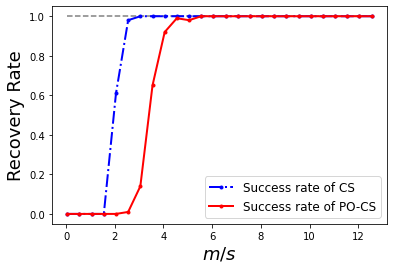
Displaying now the success rates, by counting how many times over the number of trials, the reconstruction SNR was above a certain threshold success_score (e.g., 60 dB)
success_score = 60
cslin_success = np.sum(scores_lin>success_score,axis=1)/nb_trials
cspo_success = np.sum(scores_po>success_score,axis=1)/nb_trials

mlin_tr = np.where(cslin_success > 0.5)[0][0]
mpo_tr = np.where(cspo_success > 0.5)[0][0]

print(f"m/k: CS {m_vec[mlin_tr]/k}; PO-CS {m_vec[mpo_tr]/k}")
print(f"PO-CS/CS: {m_vec[mpo_tr]/m_vec[mlin_tr]}")
print(f"mCS = {m_vec[mlin_tr]}, mPO = {m_vec[mpo_tr]}, 2*mCS - 2 = {2*m_vec[mlin_tr]-2}")

plt.figure()
plt.plot(m_vec/k, cspo_success*0 + 1.0, '--', color='gray')
plt.plot(m_vec/k, cslin_success, 'b.-.',linewidth=2, label='Success rate of CS')
plt.plot(m_vec/k, cspo_success, 'r.-',linewidth=2, label='Success rate of PO-CS')

plt.legend(fontsize=12)
#plt.title('Basis Pursuit Recovery Rates')
plt.xlabel('$m/s$',fontsize=18)
#plt.xlim((0,70/k))
plt.ylabel('Recovery Rate',fontsize=18)
#plt.savefig('BP_rec_rate_Gaussian.pdf', bbox_inches='tight', pad_inches=0.025, transparent=True)
m/k: CS 2.05; PO-CS 3.55
PO-CS/CS: 1.7317073170731707
mCS = 41, mPO = 71, 2*mCS - 2 = 80


Text(0, 0.5, 'Recovery Rate')
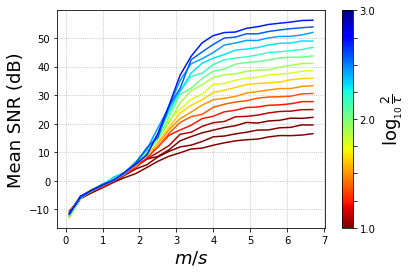
2. Noisy PO-CS reconstruction
We now consider a noisy PO-CS model described by
$$ \boldsymbol z = {\rm sign}_{\mathbb C}(\boldsymbol \Phi \boldsymbol x) + \boldsymbol \xi, \tag{PO-CS} $$
with $\boldsymbol \xi \in \mathbb C^m$ an additive noise with bounded amplitude, i.e., such that $ |\boldsymbol \xi|_\infty \leq \tau $.
Note that $\tau < 2$ since there exists a counterexample of additive noise with $|\boldsymbol \xi|_\infty \leq 2$ that totally remove any information about the signal in the phase (that is, the random dephasing, see the paper).
# Sensing model
sensing_model = 'gaussian'

# Problem dimensions
n = 100
k = 10
m_vec = np.arange(1,70,3)


# Levels of noise
nb_tau = 16
tau_vec = 2*np.logspace(-3, -1, nb_tau)

# Number of trials
nb_trials = 100

# Inits
scores_po = np.zeros((m_vec.size,nb_tau,nb_trials))

# Main Monte Carlo Loops
pbar = tqdm(total=m_vec.size) #comment this if it doesn't work for you
for m_ind, m in enumerate(m_vec):

    # The measurement vector e_1 such that A_z x0 = e_1
    e_1 = generate_canonic_vec(m+2,0)

    for s in np.arange(nb_trials):

        for t, tau in enumerate(tau_vec):

            # Generating the complex uniform noise with tau variations
            rho = np.sqrt(np.random.uniform(0, 1, m))
            phi = np.random.uniform(0, 2*np.pi, m)
            xi = tau * rho * (np.cos(phi) + np.sin(phi)*1j)

            # Generating the sensing matrix according to the selected model
            A = generate_sensing_mtx(m, n, model = sensing_model)

            # Generating a k-sparse signal, random k-length support, and Gaussian entries
            x = generate_sparse_sig(k,n)

            # linear measurements
            y = A @ x

            # phase only measurements
            z = signc(y) + xi

            # Let x0 such that ||Ax0||_1 = kappa sqrt(m) (see [1])
            # This is the signal we hope to estimate, as the amplitude of x is lost (see [1])
            x0 = x * kappa * np.sqrt(m) / np.linalg.norm(y,1)

            # Definition of the matrix A_z for sparse signal recovery in PO-CS, such that A_z x0 = (1, 0, ..., 0)
            A_z = generate_Az(A,z)

            # Defining A_xi to compute varepsilon, the level of noise
            A_xi = generate_Az(A,xi)
            varepsilon = np.linalg.norm(A_xi @ x0)

            # Phase-only model
            x_pocs = bpdnalg(A_z, e_1, varepsilon)

            # Recording SNRs
            #scores_lin[m_ind,t,s] = snr(x_lin,x0)
            scores_po[m_ind,t,s] = snr(x_pocs,x0)

    pbar.update(1) #comment this if it doesn't work for you

pbar.close() #comment this if it doesn't work for you
0%| | 0/23 [00:00<?, ?it/s]
Let’s plot the result.
mean_snr = scores_po.mean(axis=2)

fig, ax = plt.subplots(1)

# setup the normalization and the colormap
normalize = mcolors.Normalize(vmin=np.log10(tau_vec.min()/2), vmax=np.log10(tau_vec.max()/2))
colormap = cm.jet

#colors = plt.cm.magma(np.linspace(0,1,2*nb_tau))

for t in np.flip(np.arange(nb_tau)):
    ax.plot(m_vec/k, mean_snr[:,t], color=colormap(normalize(np.log10(tau_vec[t]))))

# Displaying a grid
ax.grid(linestyle=':')

# setup the colorbar
scalarmappaple = cm.ScalarMappable(norm=normalize, cmap=colormap)
scalarmappaple.set_array(20)
cbar = plt.colorbar(scalarmappaple)
cbar.ax.invert_yaxis()
cbar.set_label(r'$\log_{_{10}}\, \frac{2}{\tau}$', fontsize=18)
cbar.ax.set_yticklabels(['3.0','','','','2.0','','','','1.0'])

#plt.legend(('$\pi$/1000','$\pi$/100','$\pi$/10'))
#plt.title('Basis Pursuit Recovery Rates')
ax.set_xlabel(r'$m/s$', fontsize=18)
ax.set_ylabel('Mean SNR (dB)', fontsize=18)


#fig.colorbar

plt.savefig('BPDN_mean_snr.pdf', bbox_inches='tight', pad_inches=0, transparent=True)
<ipython-input-42-bd2bab08cf7d>:23: UserWarning: FixedFormatter should only be used together with FixedLocator
  cbar.ax.set_yticklabels(['3.0','','','','2.0','','','','1.0'])