Some comments on the Noiselet Transform (special “LazyLinopt update”)
Updates:
- (22/04/26) Great news!! A fast, butterfly (aka FFT-like), implementation of the Noiselet Transform (see below) is now integrated into the LazyLinop toolbox – “a python toolbox to ease and accelerate computations with (“matrix-free”) linear operators.” Thank you to Pascal Carrivain and Rémi Gribonval from the OCKHAM/INRIA team, in ENS Lyon, France (where I’m currently invited for a sabbatical year in 25-26) for this implementation. The idea came from common discussions we had together (I share my office with Pascal at ENS Lyon) about possible additional butterfly transformations to complete the (already long) list of operators integrated to LazyLinop. The whole Noiselet Tansform (and its inverse) is described here in the LazyLinop documentation, with a demonstration code in python. Enjoy!

- (12/03/25): I have quickly rewritten my original matlab code for computing the forward and inverse Noiselet transforms into Python. This code is available here on GitLab. It is not optimized and can certainly be largely improved.
Recently, a friend of mine asked me few questions about Noiselets for Compressed Sensing applications, i.e., in order to create efficient sensing matrices incoherent with signals which are sparse in the Haar/Daubechies wavelet basis. It seems that some of the answers are difficult to find on the web (but I’m sure they are well known to specialists) and I have therefore decided to share the ones I got.
Context: I wrote in 2008 a tiny Matlab toolbox (see here) to convince myself that the Noiselet followed a Cooley-Tukey implementation already followed by the Walsh-Hadamard transform. It should have been optimized in C but I lacked time to write this.Since this first code, I realized that Justin Romberg wrote already in 2006 with Peter Stobbe a fast code (also \(O(N \log N)\) but much faster than mine) available here.
People could be interested in using Justin’s code since, as it will be clarified from my answers given below, it is already adapted to real-valued signals, i.e., it produces real valued noiselets coefficients.
Q1. Do we need to use both the real and imaginary parts of noiselets to design sensing matrices (i.e., building the \(\Phi\) matrix)? Can we use just the real part or just the imaginary part)? Any reason why you’d do one thing or another?
As for the Random Fourier Ensemble sensing, what I personally do when I use noiselet sensing is to pick uniformly at random \(M/2\) complex values in half the noiselet-frequency domain, and concatenate the real and the imaginary part into a real vector of length \(M=2*M/2\). The adjoint (transposed) operation – often needed in most of Compressed Sensing solvers – must, of course, sum the previously split real and imaginary parts into \(M/2\) complex values before to pad the complementary measured domain with zeros and run the inverse noiselet transform.
To understand the special treatment of the real and the imaginary parts (and not simply by considering it similar to what is done for Random Fourier Ensemble), let us consider the origin, that is, Coifman et al. Noiselets paper.
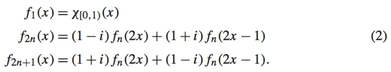
Recall that in this paper, two kinds of noiselets are defined. The first basis, the common Noiselets basis on the interval \([0, 1]\), is defined thanks to the recursive formulas:
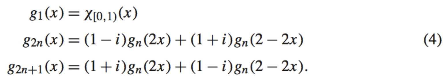
The second basis, or Dragon Noiselets, is slightly different. Its elements are symmetric under the change of coordinates \(x \to 1-x\). Their recursive definition is
To be more precise, the two sets
\[\{f_j: 2^N\leq j < 2^{N+1}\},\] \[\{g_j: 2^N\leq j < 2^{N+1}\},\]
are orthonormal bases for piecewise constant functions at resolution \(2^N\), that is, for functions of
\[V_N = \{h(x): h\ \textrm{is constant over each}\big[2^{{-N}k,2}{-N}(k+1)\big), 0\leq k < 2^N \}.\]
In Coifman et al.paper, the recursive definition of Eq. (2) (and also Eq (4) for Dragon Noiselets), which connects the noiselet functions between the noiselet index \(n\) and indices \(2n\) or \(2n+1\), is simply a common butterfly diagram that sustains the Cooley-Tukey implementation of the Noiselet transform.
The coefficients involved in Eqs (2) and (4) are simply \(1 \pm i\), which are, of course, complex conjugate of each other.
Therefore, in the Noiselet transform \(\hat X\) of a real vector \(X\) of length \(2^N\) (in one-to-one correspondence with the piecewise constant functions of \(V_N\)) involving the noiselets of indices \(n \in \{2^N, …, 2^{N+1}-1\}\), the resulting decomposition diagram is fully symmetric (with a complex conjugation) under a flip of indices \(k \leftrightarrow k’ = 2^N - 1 - k\), for \(k = 0,\, \cdots, 2^N -1\).
This shows that \[\hat X_k = \hat X^*_{k’},\] with \({(\cdot)}^*\) the complex conjugation, if \(X\) is real, and allows us to define “Real Random Noiselet Ensemble” by picking uniformly at random \(M/2\) complex values in the half domain \(k = 0,\,\cdots, 2^{N-1}-1\), that is \(M\) independent real values in total, as obtained by concatenating the real and the imaginary parts (see above).
Therefore, for real valued signals, as for Fourier, the two halves of the noiselet spectrum are not independent, and therefore, only one half is necessary to perform useful CS measurements. Justin’s code is close to this interpretation by using a real valued version of the symmetric Dragon Noiselets described in the initial Coifman et al.paper.
Q2. Are noiselets always binary? or do they take +1, -1, 0 values like Haar wavelets?
Actually, a noiselet of index \(j\) take the complex values \(2^{j} (\pm 1 \pm i)\), never \(0\).This can be easily seen from the recursive formula of Eq. (2).
They also fill the whole interval \([0, 1]\).
Update – 26/8/2013: I was obviously wrong above on the values that noiselets can take (Thank you to Kamlesh Pawar for the detection).
Noiselet amplitude can never be zero. However, either the real part or the imaginary part (not both) can vanish for certain \(n\).
So, to be correct and from few computations, a noiselet of index \(2^n + j\) with \(0 \leq j < 2^n\) takes, over the interval \([0,1]\), the complex values \(2^{(n-1)/2} (\pm 1 \pm i)\) if \(n\) is odd, and \(2^{n/2} (\pm 1)\) or \(2^{n/2} (\pm i)\) if \(n\) is even.
In particular, we see that the amplitude of these noiselets is always \(2^{n/2}\) for the considered indexes.
Q3. Walsh functions have the property that they are binary and zero mean, so that one half of the values are 1 and the other half are -1. Is it the same case with the real and/or imag parts of the noiselet transform?
To be correct, Walsh-Hadamard functions have mean equal to 1 if their index is a power of 2 and 0 else, starting with the [0,1] indicator function of index 1.
For Noiselets, they are all of unit average, meaning that the imaginary part has the zero average property. This can be proved easily (by induction) from their recursive definition in Coifman et al.paper (Eqts (2) and (4)). Interestingly, their unit average, that is their projection on the unit constant function, shows directly that a constant function is not sparse at all in the noiselet basis since its “noiselet spectrum” is just flat.
In fact, it is explained in Coifman paper that any Haar-Walsh wavelet packets, that is, elementary functions of formula \[W_n(2^q x - k),\] with \(W_n\) the Walsh functions (including the Haar functions), have a flat noiselet spectrum (all coefficients of unit amplitude), leading to the well-known good (in)coherence results (that is, low coherence). To recall, the coherence is given by \(1\) for the Haar wavelet basis, and it corresponds to slightly higher values for the Daubechies wavelets D4 and D8 respectively (see, e.g., E.J. Candès and M.B. Wakin, “An introduction to compressive sampling”, IEEE Sig. Proc. Mag., 25(2):21–30, 2008.)
Q4. How come noiselets require \(O(N \log N)\) computations rather than \(O(N)\) like the Haar transform?
This is a very common confusion. The difference comes from the locality of the Haar basis elements.
For the Haar transform, you can use the well known pyramidal algorithm running in \(O(N)\) computations. You start from the approximation coefficients computed at the finest scale, using then the wavelet scaling relations to compute the detail and approximation coefficients at the second scale, and so on. Because of the sub-sampling occuring at each scale, the complexity is proportional to the number of coefficients, that is, it is \(O(N)\).
For the 3 bases Hadamard-Walsh, Noiselets and Fourier, their non-locality (i.e., their support is the whole segment [0, 1]) you cannot run a similar algorithm. However, you can use the Cooley-Tukey algorithm arising from the Butterfly diagrams linked to the corresponding recursive definitions (Eqs (2) and (4) above).
This one is in \(O(N \log N)\), since the final diagram has \(\log_2 N\) levels, each involving \(N\) operations (multiplication-addition). — Feel free to comment on this post and ask other questions. It will provide perhaps eventually a general Noiselet FAQ/HOWTO ;-)