Quasi-isometric embeddings of vector sets with quantized sub-Gaussian projections
\(\newcommand{\cl}{\mathcal}\newcommand{\bb}{\mathbb}%\)
Last January, I was honored to be invited in RWTH Aachen University by Holger Rauhut and Sjoerd Dirksen to give a talk on the general topic of quantized compressed sensing. In particular, I decided to focus my presentation on the quasi-isometric embeddings arising in 1-bit compressed sensing, as developed by a few researchers in this field (e.g., Petros Boufounos, Richard Baraniuk, Yaniv Plan, Roman Vershynin and myself).
In comparison with isometric (bi-Lipschitz) embeddings suffering only from a multiplicative distortion, as for the restricted isometry property (RIP) for sparse vectors sets or Johnson-Lindenstrauss Lemma for finite sets, a quasi-isometric embedding \(\bf E: \mathcal K \to \mathcal L\) between two metric spaces \((\mathcal K, d_{\mathcal K})\) and \((\mathcal L,d_{\mathcal L})\) is characterized by both a multiplicative and an additive distortion, i.e., for some values \(\Delta_{\oplus},\Delta_{\otimes}>0\), \(\bf E\) respects
\[(1- \Delta_{\otimes}) d_{\mathcal K}(\boldsymbol u, \boldsymbol v) - \Delta_\oplus\leq d_{\mathcal L}(\bf E(\boldsymbol u), \bf E(\boldsymbol v)) \leq (1 + \Delta_{\otimes}) d_{\mathcal K}(\boldsymbol u, \boldsymbol v)+\Delta_\oplus,\]
for all \(\boldsymbol u,\boldsymbol v \in \mathcal K\).
In the case of 1-bit Compressed Sensing, one observes a quasi-isometric relation between the angular distance of two vectors (or signals) in \(\mathbb R^N\) and the Hamming distance of their 1-bit quantized projections in \(\{\pm 1\}^M\). This mapping is simply obtained by keeping the sign (componentwise) of their multiplication by a \(M \times N\) random Gaussian matrix Mathematically,
\[\boldsymbol{A}_{\rm 1bit} : \boldsymbol{u} \in \mathbb R^{N}$ \mapsto \boldsymbol{A}_{\rm 1bit}(\boldsymbol{u}) := {\rm sign}(\boldsymbol{\Phi} \boldsymbol{u})\]
with \(\boldsymbol\Phi \in \mathbb R^{M\times N}\) and \(\Phi_{ij} \sim_{\rm iid} \mathcal N(0,1)\). Notice that for a general sensing matrix (e.g., possibly non-Gaussian), if reachable, \({\bf A}_{1bit}\) can only induce a quasi-isometric relation. This is due to the information loss induced by the “sign” quantization in, e.g., the loss of the signal amplitude. Moreover, it is known that for a Bernoulli sensing matrix \(\boldsymbol \Phi \in \{\pm 1\}^{M \times N}\), two vectors can be arbitrarily close and share the same quantization point [2,5]. Interestingly, it has been shown in a few works that quasi-isometric 1-bit embeddings exist for \(K\)-sparse signals [1] or for any bounded subset \(\mathcal K\) of \(\mathbb R^N\) provided the typical dimension of this set is bounded [2]. This dimension is nothing but the Gaussian mean width \(w(\mathcal K)\) of the set [2] defined by
\[w(\mathcal K) = \mathbb E \sup_{\boldsymbol u \in \mathcal K} |\boldsymbol g^T \boldsymbol u|,\quad \boldsymbol g \sim \mathcal N(0,{\rm Id}_N).\]
Since the 80’s, this dimension has been recognized as central for instance in characterizing random processes [9], shrinkage estimators in signal denoising and high-dimensional statistics [10], linear inverse problem solving with convex optimization [11] or classification efficiency in randomly projected signal sets [12]. Moreover, for the set of bounded K-sparse signals, we have \(w(\mathcal K)^2 \leq C K \log N/K\), which is the quantity of interest for characterizing the RIP of order \(K\) of random Gaussian matrices (with other interesting characterizations for the compressible signals set or for “signals” consisting of rank-r matrices). In [2], by connecting the problem to the context of random tessellation of the sphere \(\mathbb S^{N-1}\), the authors have shown that if \(M\) is larger than \(M \geq C \epsilon^{-6} w(\mathcal K)^2\), then, for all \(x,y \in \mathcal K\),
\[d_{\rm ang}(x,y) - \epsilon \leq d_H(\boldsymbol A_{\rm 1bit}(x), \boldsymbol A_{\rm 1bit}(y)) \leq d_{\rm ang}(x,y) \epsilon.\]
For \(K\)-sparse vectors, this condition is even reduced to \(M=O(\epsilon^{-2} K \log N/K)\) as shown in [1]. As explained in my previous post on quantized embedding and the funny connection with Buffon’s needle problem, I have recently noticed that for finite sets \(\mathcal K \subset \mathbb R^N\), quasi-isometric relations also exist with high probability between the Euclidean distance (or \(\ell_2\)-distance) of vectors and the \(\ell_1\)-distance of their (dithered) quantized random projections. Generalizing \({\bf A}_{\rm 1bit}\) above, this new mapping reads \({\bf A}: \boldsymbol u \in \mathbb R^N \mapsto \mathcal {\bf A}(\boldsymbol u) := Q(\boldsymbol \Phi\boldsymbol u \boldsymbol \xi) \in \delta \mathbb Z^M\), for a (“round-off”) scalar quantizer \(\mathcal Q(\cdot) = \delta \lfloor \cdot / \delta \rfloor\) with resolution \(\delta>0\) applied componentwize on vectors, a random Gaussian \(\boldsymbol \Phi\) (as above) and a dithering \(\boldsymbol \xi \in \mathbb R^{M}\), with \(\xi_i \sim_{\rm iid} \mathcal U([0,\delta])\) uniformizing the action of the quantizer (as used in [6] for more general quantizers). In particular, provided \(M \geq C \epsilon^{-2}\log |\mathcal K|\), with high probability, for all \(\boldsymbol x, \boldsymbol y \in \mathcal K\),
\[(\sqrt{\frac{2}{\pi}} - \epsilon)\|\boldsymbol x - \boldsymbol y\| - c\delta\epsilon \leq \frac{1}{M}\|\boldsymbol A(\boldsymbol x) - \boldsymbol A(\boldsymbol y)\|_1 \leq (\sqrt{\frac{2}{\pi}}+\epsilon)\|\boldsymbol x - \boldsymbol y\| + c\delta\epsilon,\qquad(1)\]
for some general constants \(C,c>0\).
One observes that the additive distortion of this last relation reads \(\Delta_\oplus = c\delta\epsilon\), i.e., it can be made arbitrarily low with \(\epsilon\)! However, directly integrating the quantization in the RIP satisfied by \(\boldsymbol \Phi\) would have rather led to a constant additive distortion, only function of \(\delta\).
Remark: For information, as provided by an anonymous expert reviewer, it happens that a much shorter and elegant proof of this fact exists using the sub-Gaussian properties of the quantized mapping \(\bf A\) (see Appendix A in the associated revised paper).
In that work, the question remained, however, on how to extend (1) for vectors taken in any (bounded) subset \(\mathcal K\) of \(\mathbb R^N\), hence generalizing the quasi-isometric embeddings observed for 1-bit random projections? Moreover, it was still unclear if the sensing matrix \(\boldsymbol \Phi\) could be non-Gaussian, i.e., if any sub-Gaussian matrix (e.g., Bernoulli \(\pm 1\)) could define a suitable $\bf A.$
While I was in Aachen discussing with Holger and Sjoerd during and after my presentation, I realized that the works [2-5] of Plan, Verhsynin, Ai and collaborators provided already many important tools whose adaptation to the mapping \(\bf A\) above could answer those questions.
At the heart of [2] lies the equivalence between
\[d_H(\boldsymbol A_{\rm 1bit}(\boldsymbol x), \boldsymbol A_{\rm 1bit}(\boldsymbol y))\]
and a counting procedure associated to
\[\textstyle d_H(\boldsymbol A_{\rm 1bit}(\boldsymbol x), \boldsymbol A_{\rm 1bit}(\boldsymbol y)) = \frac{1}{M} \sum_i \mathbb I[\mathcal E (\boldsymbol \varphi_i^T \boldsymbol x, \boldsymbol \varphi_i^T \boldsymbol y)],\]
where \(\boldsymbol \varphi_i\) is the \(i^{\rm th}\) row of \(\boldsymbol \Phi\), \(\mathbb I(A)\) is the indicator set function equals to 1 if \(A\) is non-empty and 0 otherwise, and
\[\mathcal E(a,b) = \{{\rm sign}(a) \neq {\rm sign}(b)\}.\]
In words, \(d_H(\boldsymbol A_{\rm 1bit}(\boldsymbol x), \boldsymbol A_{\rm 1bit}(\boldsymbol y))\) counts the number of hyperplanes defined by the normals \(\boldsymbol \varphi_i\) that separate \(\boldsymbol x\) from \(\boldsymbol y\).
Without giving too many details in this post, the work [2] leverages this equivalence to make a connection with tessellation of the \((N-1)\)-sphere where it is shown that the number of such separating random hyperplanes is somehow close (up to some distortions) to the angular distance between the two vecors. They obtain this by “softening” the Hamming distance above, i.e., by introducing, for some \(t \in \mathbb R\), the soft Hamming distance
\[d^t_H(\boldsymbol A_{\rm 1bit}(\boldsymbol x), \boldsymbol A_{\rm 1bit}(\boldsymbol y)) := \frac{1}{M} \sum_i \mathbb I[\mathcal F^t(\boldsymbol \varphi_i^T \boldsymbol x, \boldsymbol \varphi_i^T \boldsymbol y)],\]
with now
\[\mathcal F^t(a,b) = \{a > t, b \leq -t\} \cup \{a \leq -t, b > t\}.\]
This distance has an interesting continuity property compared to \(d_H = d^0_H\). In particular, if one allows \(t\) to vary, it is continuous up to small (\(\ell_1\)) perturbations of \(\boldsymbol x\) and \(\boldsymbol y\).
In our context, considering the quantized mapping \(\bf A\) specified above, we can define the generalized soften distance :
\[\textstyle \mathcal Q^t(\boldsymbol x,\boldsymbol y) := \tfrac{\delta}{M}\sum_{i=1}^M \sum_{k\in\mathbb Z} \mathbb I[\mathcal F^t(\boldsymbol \varphi_i^T \boldsymbol x + \xi_i - k\delta, \boldsymbol \varphi_i^T \boldsymbol y + \xi_i - k\delta)].\]
When \(t=0\) we actually recover the distance used in the quasi-isometry (1), i.e.,
\[\textstyle \mathcal Q^0(\boldsymbol x,\boldsymbol y) = \frac{1}{M} \|\boldsymbol A(\boldsymbol x) - \boldsymbol A(\boldsymbol y)\|_1,\]
similarly to the recovering of the Hamming distance in 1-bit case.
The interpretation of \(\mathcal Q^t(\boldsymbol x,\boldsymbol y)\) when \(t=0\) is now that we again count the number of hyperplanes defined by the normals \(\boldsymbol \varphi_i\) that separate \(\boldsymbol x\) from \(\boldsymbol y\), but now, for each measurement index \(1 \leq i \leq M\) this count can be bigger than 1 as we allow multiple parallel hyperplanes for each normal \(\boldsymbol \varphi_i\), all \(\delta\) far apart. This is in connection with the “hyperplane wave partitions’’ defined in [7,8], e.g., for explaining quantization of vector frame coefficients. As explained in the paper, when \(t\neq 0\), then \(\mathcal Q^t\) relaxes (for \(t < 0\)) or strengthens (for \(t \geq 0\)) the conditions allowing to count a separating hyperplane.
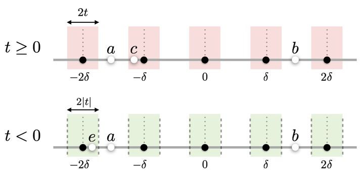
Remark: The picture featured on the top of this page represents the behavior of \(d^{t}(a,b) := \mathcal Q^t(a,b)\), that is \(Q^{t}\) in one-dimension for \(\boldsymbol \varphi_i = 1\) and \(a,b \in \mathbb R\) (see page Fig. 1, p. 16 of the paper for more explanation). On the top, \(t\geq 0\) and forbidden areas determined by \(\cl F^t\) are created when counting the number of thresholds \(k\delta\) separating \(a\) and \(b\). For instance, for an additional point \(c\in \mathbb R\) as on the figure, \(d^0(a,b)=d^0(c,b)=3\delta\) but \(3\delta=d^t(a,b)=d^t(c,b)+\delta \geq d^t(c,b)\) as \(c\) lies in one forbidden area. On the bottom figure, \(t\leq 0\) and threshold counting procedure operated by \(d^t\) is relaxed. Now \(d^t(a,b)\) counts the number of limits (in dashed) of the green areas determined by \(\cl F^t\), recording only one per thresholds \(k\delta\), that separate \(a\) and \(b\). Here, for \(e\in \mathbb R\) as on the figure, \(d^0(a,b)=d^0(e,b)=3\delta\) but \(4\delta=d^t(e,b)=d^t(a,b) +\delta \geq d^t(a,b)\).
As for 1-bit projections, we can show the continuity of \(\mathcal Q^t(\boldsymbol x,\boldsymbol y)\) with respect to small (\(\ell_2\) now) perturbation of \(\boldsymbol x\) and \(\boldsymbol y\), and this fact allows to study the random (sub-Gaussian) concentration of \(\mathcal Q^t(\boldsymbol x,\boldsymbol y)\), i.e., studying it for a coverage of the set of interest, and then extending it to the whole set from this continuity. From this observation, and after a few months of works, I have gathered all these developments in the following paper, now submitted on arxiv:
Briefly, benefiting of the context defined above, this work contains two main results. First, it shows that given a symmetric sub-Gaussian distribution \(\varphi\) and a precision \(\epsilon > 0\), if
\[M \geq C \epsilon^{-5} w(\mathcal K)^2\]
and if the sensing matrix \(\boldsymbol \Phi\) has entries i.i.d. as \(\varphi\), then, with high probability, the mapping \(\bf A\) above provides a \(\ell_2/\ell_1\)-quasi-isometry between vector pair of \(\mathcal K\) whose difference are “not too sparse” (as already noticed in [5] for 1-bit CS) and their images in \(\delta \mathbb Z^M\). More precisely, for some \(c >0\), if for \(K_0 >0\),
\[\boldsymbol x - \boldsymbol y \in C_{K_0} = \{\boldsymbol u \in \mathbb R^N: K_0\|\boldsymbol u\|^2_\infty \leq \|\boldsymbol u\|^2\}\]
then, given some constant \(\kappa_{\rm sg}\) depending on the sub-Gaussian distribution \(\varphi\) (with \(\kappa_{\rm sg} = 0\) if \(\varphi\) is Gaussian),
\[\textstyle {(\sqrt{\frac{2}{\pi}} - \epsilon - \frac{\kappa_{\rm sg}}{\sqrt K_0}) \|\boldsymbol x - \boldsymbol y\|- c\epsilon\delta\ \leq\ \frac{1}{M} \|\boldsymbol A(\boldsymbol x) - \boldsymbol A(\boldsymbol y)\|_1\ \leq\ (\sqrt{\frac{2}{\pi}} + \epsilon + \frac{\kappa_{\rm sg}}{\sqrt K_0}) \|\boldsymbol x - \boldsymbol y\|+c\epsilon\delta.}\]
Interestingly, in this quasi-isometric embedding, we notice that the additive distortion is driven by \(\epsilon\delta\) as in (1) while the multiplicative distortion reads now
\[\Delta_{\otimes} = \epsilon + \frac{\kappa_{\rm sg}}{\sqrt K_0}.\]
In addition to its common dependence in the precision \(\epsilon\), this distortion is also function of the “antisparse” nature of \(\boldsymbol x - \boldsymbol y\). Indeed, if \(\boldsymbol u \in C_{K_0}\) then it cannot be sparser than \(K_0\) with anyway \(C_{K_0} \neq \mathbb R^N \setminus \Sigma_{K_0}\). In other words, when the matrix \(\boldsymbol \Phi\) is non-Gaussian (but sub-Gaussian anyway), the distortion is smaller for “anti-sparse” vector differences.
In the particular case where \(\mathcal K\) is the set of bounded \(K\)-sparse vectors in any orthonormal basis, then only
\[ M \geq C \epsilon^{-2} \log(c N/K\epsilon^{3/2}) \]
measurements suffice for defining the same embedding with high probability. As explained in the paper, this case allows somehow to mitigate the anti-sparse requirement as sparse vectors in some basis can be made less sparse in another, e.g., for dual bases such as DCT/Canonical, Noiselet/Haar, etc.
The second result concerns the consistency width of the mapping \(A\), i.e., the biggest distance separating distinct vectors that are projected by \(A\) on the same quantization point. With high probability, it happens that the consistency width \(\epsilon\) of any pair of vectors whose difference is again``not too sparse’’ decays as
\[\epsilon = O(M^{-1/4}w(\mathcal K)^{1/2})\]
for a general subset \(\mathcal K\) and, up to some log factors, as \(\epsilon = M^{-1}\) for sparse vector sets.
Open problem: I’m now wondering if the tools and results above could be extended to other quantizers \(\mathcal Q\), such as the universal quantizer defined in [6]. This periodic quantizer has been shown to provide exponentially decaying distortions [6,13] for embedding of sparse vectors, with interesting applications (e.g., information retrieval). Knowing if this holds for other vector sets and for other (sub-Gaussian) sensing matrix is an appealing open question.
References:
- [1] L. Jacques, J. N. Laska, P. T. Boufounos, and R. G Baraniuk. “Robust 1-bit compressive sensing via binary stable embeddings of sparse vectors”. IEEE Transactions on Information Theory, 59(4):2082–2102, 2013.
- [2] Y. Plan and R. Vershynin. “Dimension reduction by random hyperplane tessellations”. Discrete & Computational Geometry, 51(2):438–461, 2014, Springer.
- [3] Y. Plan and R. Vershynin. “Robust 1-bit compressed sensing and sparse logistic regression: A convex programming approach”. IEEE Transactions on Information Theory, 59(1): 482–494, 2013.
- [4] Y. Plan and R. Vershynin. “One-bit compressed sensing by linear programming”. Communications on Pure and Applied Mathematics, 66(8):1275–1297, 2013.
- [5] A. Ai, A. Lapanowski, Y. Plan, and R. Vershynin. “One-bit compressed sensing with non-gaussian measurements”. Linear Algebra and its Applications, 441:222–239, 2014.
- [6] P. T. Boufounos. Universal rate-efficient scalar quantization. IEEE Trans. Info. Theory, 58(3):1861–1872, March 2012.
- [7] V. K Goyal, M. Vetterli, and N. T. Thao. Quantized overcomplete expansions in \(\mathbb R^N\) : Analysis, synthesis, and algorithms. IEEE Trans. Info. Theory, 44(1):16–31, 1998.
- [8] N. T . Thao and M. Vetterli. “Lower bound on the mean-squared error in oversampled quantization of periodic signals using vector quantization analysis”. IEEE Trans. Info. Theory, 42(2):469–479, March 1996.
- [9] A. W. Vaart and J. A. Wellner. Weak convergence and empirical processes. Springer, 1996.
- [10] V. Chandrasekaran and M. I. Jordan. Computational and statistical tradeoffs via convex relaxation. arXiv preprint arXiv:1211.1073, 2012.
- [11] V. Chandrasekaran, B. Recht, P. A Parrilo, and A. S. Willsky. The convex geometry of linear inverse problems. Foundations of Computational mathematics, 12(6):805–849, 2012.
- [12] A. Bandeira, D. G Mixon, and B. Recht. Compressive classification and the rare eclipse problem. arXiv preprint arXiv:1404.3203, 2014.
- [13] P. T. Boufounos and S. Rane. Efficient coding of signal distances using universal quantized embeddings. In Proc. Data Compression Conference (DCC), Snowbird, UT, March 20-22 2013.